API

Index

Survey.AbstractSurveyDesign
Survey.BootstrapReplicates
Survey.JackknifeReplicates
Survey.ReplicateDesign
Survey.SurveyDesign
GLM.glm
Statistics.mean
Statistics.quantile
Survey.bootweights
Survey.boxplot
Survey.freedman_diaconis
Survey.hist
Survey.jackknifeweights
Survey.load_data
Survey.plot
Survey.ratio
Survey.standarderror
Survey.sturges
Survey.total

Survey.AbstractSurveyDesign — Type

AbstractSurveyDesign

Supertype for every survey design type.

Note

The data passed to a survey constructor is modified. To avoid this pass a copy of the data instead of the original.

source

Survey.SurveyDesign — Type

SurveyDesign <: AbstractSurveyDesign

General survey design encompassing a simple random, stratified, cluster or multi-stage design.

In the case of cluster sample, the clusters are chosen by simple random sampling. All individuals in one cluster are sampled. The clusters are considered disjoint and nested.

strata and clusters must be given as columns in data.

Arguments:

data::AbstractDataFrame: the survey dataset (!this gets modified by the constructor).
strata::Union{Nothing, Symbol}=nothing: the stratification variable.
clusters::Union{Nothing, Symbol, Vector{Symbol}}=nothing: the clustering variable.
weights::Union{Nothing, Symbol}=nothing: the sampling weights.
popsize::Union{Nothing, Symbol}=nothing: the (expected) survey population size.

julia> apiclus1 = load_data("apiclus1");

julia> dclus1 = SurveyDesign(apiclus1; clusters=:dnum, weights=:pw)
SurveyDesign:
data: 183×44 DataFrame
strata: none
cluster: dnum
    [637, 637, 637  …  448]
popsize: [507.7049, 507.7049, 507.7049  …  507.7049]
sampsize: [15, 15, 15  …  15]
weights: [33.847, 33.847, 33.847  …  33.847]
allprobs: [0.0295, 0.0295, 0.0295  …  0.0295]

source

Survey.ReplicateDesign — Type

ReplicateDesign <: AbstractSurveyDesign

Survey design obtained by replicating an original design using an inference method like bootweights or jackknifeweights. If replicate weights are available, then they can be used to directly create a ReplicateDesign object.

Constructors

ReplicateDesign{ReplicateType}(
    data::AbstractDataFrame,
    replicate_weights::Vector{Symbol};
    clusters::Union{Nothing,Symbol,Vector{Symbol}} = nothing,
    strata::Union{Nothing,Symbol} = nothing,
    popsize::Union{Nothing,Symbol} = nothing,
    weights::Union{Nothing,Symbol} = nothing
) where {ReplicateType <: InferenceMethod}

ReplicateDesign{ReplicateType}(
    data::AbstractDataFrame,
    replicate_weights::UnitIndex{Int};
    clusters::Union{Nothing,Symbol,Vector{Symbol}} = nothing,
    strata::Union{Nothing,Symbol} = nothing,
    popsize::Union{Nothing,Symbol} = nothing,
    weights::Union{Nothing,Symbol} = nothing
) where {ReplicateType <: InferenceMethod}

ReplicateDesign{ReplicateType}(
    data::AbstractDataFrame,
    replicate_weights::Regex;
    clusters::Union{Nothing,Symbol,Vector{Symbol}} = nothing,
    strata::Union{Nothing,Symbol} = nothing,
    popsize::Union{Nothing,Symbol} = nothing,
    weights::Union{Nothing,Symbol} = nothing
) where {ReplicateType <: InferenceMethod}

Arguments

ReplicateType must be one of the supported inference types; currently the package supports BootstrapReplicates and JackknifeReplicates. The constructor has the same arguments as SurveyDesign. The only additional argument is replicate_weights, which can be of one of the following types.

Vector{Symbol}: In this case, each Symbol in the vector should represent a column of data containing the replicate weights.
UnitIndex{Int}: For instance, this could be UnitRange(5:10). This will mean that the replicate weights are contained in columns 5 through 10.
Regex: In this case, all the columns of data which match this Regex will be treated as the columns containing the replicate weights.

All the columns containing the replicate weights will be renamed to the form replicate_i, where i ranges from 1 to the number of columns containing the replicate weights.

Examples

Here is an example where the bootweights function is used to create a ReplicateDesign{BootstrapReplicates}.

julia> apistrat = load_data("apistrat");

julia> dstrat = SurveyDesign(apistrat; strata=:stype, weights=:pw);

julia> bootstrat = bootweights(dstrat; replicates=1000)     # creating a ReplicateDesign using bootweights
ReplicateDesign{BootstrapReplicates}:
data: 200×1044 DataFrame
strata: stype
    [E, E, E  …  H]
cluster: none
popsize: [4420.9999, 4420.9999, 4420.9999  …  755.0]
sampsize: [100, 100, 100  …  50]
weights: [44.21, 44.21, 44.21  …  15.1]
allprobs: [0.0226, 0.0226, 0.0226  …  0.0662]
type: bootstrap
replicates: 1000

If the replicate weights are given to us already, then we can directly pass them to the ReplicateDesign constructor. For instance, in the above example, suppose we had the bootstrat data as a CSV file (for this example, we also rename the columns containing the replicate weights to the form r_i).

julia> using CSV;

julia> DataFrames.rename!(bootstrat.data, ["replicate_"*string(index) => "r_"*string(index) for index in 1:1000]);

julia> CSV.write("apistrat_withreplicates.csv", bootstrat.data);

We can now pass the replicate weights directly to the ReplicateDesign constructor, either as a Vector{Symbol}, a UnitRange or a Regex.

julia> bootstrat_direct = ReplicateDesign{BootstrapReplicates}(CSV.read("apistrat_withreplicates.csv", DataFrame), [Symbol("r_"*string(replicate)) for replicate in 1:1000]; strata=:stype, weights=:pw)
ReplicateDesign{BootstrapReplicates}:
data: 200×1044 DataFrame
strata: stype
    [E, E, E  …  H]
cluster: none
popsize: [4420.9999, 4420.9999, 4420.9999  …  755.0]
sampsize: [100, 100, 100  …  50]
weights: [44.21, 44.21, 44.21  …  15.1]
allprobs: [0.0226, 0.0226, 0.0226  …  0.0662]
type: bootstrap
replicates: 1000

julia> bootstrat_unitrange = ReplicateDesign{BootstrapReplicates}(CSV.read("apistrat_withreplicates.csv", DataFrame), UnitRange(45:1044);strata=:stype, weights=:pw)
ReplicateDesign{BootstrapReplicates}:
data: 200×1044 DataFrame
strata: stype
    [E, E, E  …  H]
cluster: none
popsize: [4420.9999, 4420.9999, 4420.9999  …  755.0]
sampsize: [100, 100, 100  …  50]
weights: [44.21, 44.21, 44.21  …  15.1]
allprobs: [0.0226, 0.0226, 0.0226  …  0.0662]
type: bootstrap
replicates: 1000

julia> bootstrat_regex = ReplicateDesign{BootstrapReplicates}(CSV.read("apistrat_withreplicates.csv", DataFrame), r"r_\d";strata=:stype, weights=:pw)
ReplicateDesign{BootstrapReplicates}:
data: 200×1044 DataFrame
strata: stype
    [E, E, E  …  H]
cluster: none
popsize: [4420.9999, 4420.9999, 4420.9999  …  755.0]
sampsize: [100, 100, 100  …  50]
weights: [44.21, 44.21, 44.21  …  15.1]
allprobs: [0.0226, 0.0226, 0.0226  …  0.0662]
type: bootstrap
replicates: 1000

source

Survey.BootstrapReplicates — Type

BootstrapReplicates <: InferenceMethod

Type for the bootstrap replicates method. For more details, see bootweights.

source

Survey.JackknifeReplicates — Type

JackknifeReplicates <: InferenceMethod

Type for the Jackknife replicates method. For more details, see jackknifeweights.

source

Survey.load_data — Function

load_data(name)

Load a sample dataset as a DataFrame.

All available datasets can be found here.

julia> apisrs = load_data("apisrs")
200×40 DataFrame
 Row │ Column1  cds             stype    name             sname                ⋯
     │ Int64    Int64           String1  String15         String               ⋯
─────┼──────────────────────────────────────────────────────────────────────────
   1 │    1039  15739081534155  H        McFarland High   McFarland High       ⋯
   2 │    1124  19642126066716  E        Stowers (Cecil   Stowers (Cecil B.) E
   3 │    2868  30664493030640  H        Brea-Olinda Hig  Brea-Olinda High
   4 │    1273  19644516012744  E        Alameda Element  Alameda Elementary
   5 │    4926  40688096043293  E        Sunnyside Eleme  Sunnyside Elementary ⋯
   6 │    2463  19734456014278  E        Los Molinos Ele  Los Molinos Elementa
   7 │    2031  19647336058200  M        Northridge Midd  Northridge Middle
   8 │    1736  19647336017271  E        Glassell Park E  Glassell Park Elemen
  ⋮  │    ⋮           ⋮            ⋮            ⋮                       ⋮      ⋱
 194 │    4880  39686766042782  E        Tyler Skills El  Tyler Skills Element ⋯
 195 │     993  15636851531987  H        Desert Junior/S  Desert Junior/Senior
 196 │     969  15635291534775  H        North High       North High
 197 │    1752  19647336017446  E        Hammel Street E  Hammel Street Elemen
 198 │    4480  37683386039143  E        Audubon Element  Audubon Elementary   ⋯
 199 │    4062  36678196036222  E        Edison Elementa  Edison Elementary
 200 │    2683  24657716025621  E        Franklin Elemen  Franklin Elementary
                                                 36 columns and 185 rows omitted

source

Survey.bootweights — Function

Use bootweights to create replicate weights using Rao-Wu bootstrap. The function accepts a SurveyDesign and returns a ReplicateDesign{BootstrapReplicates} which has additional columns for replicate weights.

The replicate weight for replicate $r$ is computed using the formula $w_{i}(r) = w_i \times \frac{n_h}{n_h - 1} m_{hj}(r)$ for observation $i$ in psu $j$ of stratum $h$.

In the formula above, $w_i$ is the original weight for observation $i$, $n_h$ is the number of psus in stratum $h$, and $m_{hj}(r)$ is the number of psus in stratum $h$ that are selected in replicate $r$.

julia> using Random

julia> apiclus1 = load_data("apiclus1");

julia> dclus1 = SurveyDesign(apiclus1; clusters = :dnum, popsize=:fpc);

julia> bootweights(dclus1; replicates=1000, rng=MersenneTwister(111)) # choose a seed for deterministic results
ReplicateDesign{BootstrapReplicates}:
data: 183×1044 DataFrame
strata: none
cluster: dnum
    [61, 61, 61  …  815]
popsize: [757, 757, 757  …  757]
sampsize: [15, 15, 15  …  15]
weights: [50.4667, 50.4667, 50.4667  …  50.4667]
allprobs: [0.0198, 0.0198, 0.0198  …  0.0198]
type: bootstrap
replicates: 1000

Reference

pg 385, Section 9.3.3 Bootstrap - Sharon Lohr, Sampling Design and Analysis (2010)

source

Survey.jackknifeweights — Function

jackknifeweights(design::SurveyDesign)

Delete-1 Jackknife algorithm for replication weights from sampling weights. The replicate weights are calculated using the following formula.

\[w_{i(hj)} = \begin{cases} w_i\quad\quad &\text{if observation unit }i\text{ is not in stratum }h\\ 0\quad\quad &\text{if observation unit }i\text{ is in psu }j\text{of stratum }h\\ \dfrac{n_h}{n_h - 1}w_i \quad\quad &\text{if observation unit }i\text{ is in stratum }h\text{ but not in psu }j\\ \end{cases}\]

In the above formula, $w_i$ represent the original weights, $w_{i(hj)}$ represent the replicate weights when the $j$th PSU from cluster $h$ is removed, and $n_h$ represents the number of unique PSUs within cluster $h$. Replicate weights are added as columns to design.data, and these columns have names of the form replicate_i, where i ranges from 1 to the number of replicate weight columns.

Examples

julia> using Survey;

julia> apistrat = load_data("apistrat");

julia> dstrat = SurveyDesign(apistrat; strata=:stype, weights=:pw);

julia> rstrat = jackknifeweights(dstrat)
ReplicateDesign{JackknifeReplicates}:
data: 200×244 DataFrame
strata: stype
    [E, E, E  …  M]
cluster: none
popsize: [4420.9999, 4420.9999, 4420.9999  …  1018.0]
sampsize: [100, 100, 100  …  50]
weights: [44.21, 44.21, 44.21  …  20.36]
allprobs: [0.0226, 0.0226, 0.0226  …  0.0491]
type: jackknife
replicates: 200

Reference

pg 380-382, Section 9.3.2 Jackknife - Sharon Lohr, Sampling Design and Analysis (2010)

source

Survey.standarderror — Function

standarderror(x::Union{Symbol, Vector{Symbol}}, func::Function, design::ReplicateDesign{BootstrapReplicates}, args...; kwargs...)

Compute the standard error of the estimated mean using the bootstrap method.

Arguments

x::Union{Symbol, Vector{Symbol}}: Symbol or vector of symbols representing the variable(s) for which the mean is estimated.
func::Function: Function used to calculate the mean.
design::ReplicateDesign{BootstrapReplicates}: Replicate design object.
args...: Additional arguments to be passed to the function.
kwargs...: Additional keyword arguments.

Returns

df: DataFrame containing the estimated mean and its standard error.

The standard error is calculated using the formula

\[\hat{V}(\hat{\theta}) = \dfrac{1}{R}\sum_{i = 1}^R(\theta_i - \hat{\theta})^2\]

where above $R$ is the number of replicate weights, $\theta_i$ is the estimator computed using the $i$th set of replicate weights, and $\hat{\theta}$ is the estimator computed using the original weights.

Examples

julia> my_mean(df::DataFrame, column, weights) = StatsBase.mean(df[!, column], StatsBase.weights(df[!, weights]));

julia> Survey.standarderror(:api00, my_mean, bclus1)
1×2 DataFrame
 Row │ estimator  SE
     │ Float64    Float64
─────┼────────────────────
   1 │   644.169  23.4107

source

standarderror(x::Symbol, func::Function, design::ReplicateDesign{JackknifeReplicates})

Compute standard error of column x for the given func using the Jackknife method. The formula to compute this variance is the following.

\[\hat{V}_{\text{JK}}(\hat{\theta}) = \sum_{h = 1}^H \dfrac{n_h - 1}{n_h}\sum_{j = 1}^{n_h}(\hat{\theta}_{(hj)} - \hat{\theta})^2\]

Above, $\hat{\theta}$ represents the estimator computed using the original weights, and $\hat{\theta_{(hj)}}$ represents the estimator computed from the replicate weights obtained when PSU $j$ from cluster $h$ is removed.

Examples

julia> my_mean(df::DataFrame, column, weights) = StatsBase.mean(df[!, column], StatsBase.weights(df[!, weights]));

julia> Survey.standarderror(:api00, my_mean, rstrat)
1×2 DataFrame
 Row │ estimator  SE
     │ Float64    Float64
─────┼────────────────────
   1 │   662.287  9.53613

Reference

pg 380-382, Section 9.3.2 Jackknife - Sharon Lohr, Sampling Design and Analysis (2010)

source

Statistics.mean — Function

mean(var, design)

Estimate the mean of a variable.

julia> apiclus1 = load_data("apiclus1");

julia> dclus1 = SurveyDesign(apiclus1; clusters = :dnum, weights = :pw)
SurveyDesign:
data: 183×44 DataFrame
strata: none
cluster: dnum
    [637, 637, 637  …  448]
popsize: [507.7049, 507.7049, 507.7049  …  507.7049]
sampsize: [15, 15, 15  …  15]
weights: [33.847, 33.847, 33.847  …  33.847]
allprobs: [0.0295, 0.0295, 0.0295  …  0.0295]

julia> mean(:api00, dclus1)
1×1 DataFrame
 Row │ mean
     │ Float64
─────┼─────────
   1 │ 644.169

source

mean(x::Symbol, design::ReplicateDesign)

Compute the standard error of the estimated mean using replicate weights.

Arguments

x::Symbol: Symbol representing the variable for which the mean is estimated.
design::ReplicateDesign: Replicate design object.

Returns

df: DataFrame containing the estimated mean and its standard error.

Examples

julia> mean(:api00, bclus1)
1×2 DataFrame
 Row │ mean     SE
     │ Float64  Float64
─────┼──────────────────
   1 │ 644.169  23.4107

source

Estimate the mean of a list of variables.

julia> mean([:api00, :enroll], dclus1)
2×2 DataFrame
 Row │ names   mean
     │ String  Float64
─────┼─────────────────
   1 │ api00   644.169
   2 │ enroll  549.716

Use replicate weights to compute the standard error of the estimated means.

julia> mean([:api00, :enroll], bclus1)
2×3 DataFrame
 Row │ names   mean     SE
     │ String  Float64  Float64
─────┼──────────────────────────
   1 │ api00   644.169  23.4107
   2 │ enroll  549.716  45.7835

source

mean(var, domain, design)

Estimate means of domains.

julia> mean(:api00, :cname, dclus1)
11×2 DataFrame
 Row │ mean     cname
     │ Float64  String
─────┼──────────────────────
   1 │ 669.0    Alameda
   2 │ 472.0    Fresno
   3 │ 452.5    Kern
   4 │ 647.267  Los Angeles
   5 │ 623.25   Mendocino
   6 │ 519.25   Merced
   7 │ 710.563  Orange
   8 │ 709.556  Plumas
   9 │ 659.436  San Diego
  10 │ 551.189  San Joaquin
  11 │ 732.077  Santa Clara

Use the replicate design to compute standard errors of the estimated means.

julia> mean(:api00, :cname, bclus1)
11×3 DataFrame
 Row │ mean     SE            cname
     │ Float64  Float64       String
─────┼────────────────────────────────────
   1 │ 732.077  58.2169       Santa Clara
   2 │ 659.436   2.66703      San Diego
   3 │ 519.25    2.28936e-15  Merced
   4 │ 647.267  47.6233       Los Angeles
   5 │ 710.563   2.19826e-13  Orange
   6 │ 472.0     1.13687e-13  Fresno
   7 │ 709.556   1.26058e-13  Plumas
   8 │ 669.0     1.27527e-13  Alameda
   9 │ 551.189   2.18162e-13  San Joaquin
  10 │ 452.5     0.0          Kern
  11 │ 623.25    1.09545e-13  Mendocino

source

Survey.total — Function

total(var, design)

Estimate the population total of variable.

julia> apiclus1 = load_data("apiclus1");

julia> dclus1 = SurveyDesign(apiclus1; clusters = :dnum, weights = :pw);

julia> total(:api00, dclus1)
1×1 DataFrame
 Row │ total
     │ Float64
─────┼───────────
   1 │ 3.98999e6

source

total(x::Symbol, design::ReplicateDesign)

Compute the standard error of the estimated total using replicate weights.

Arguments

x::Symbol: Symbol representing the variable for which the total is estimated.
design::ReplicateDesign: Replicate design object.

Returns

df: DataFrame containing the estimated total and its standard error.

Examples

julia> total(:api00, bclus1)
1×2 DataFrame
 Row │ total      SE
     │ Float64    Float64
─────┼──────────────────────
   1 │ 3.98999e6  9.01611e5

source

Estimate the population total of a list of variables.

julia> total([:api00, :enroll], dclus1)
2×2 DataFrame
 Row │ names   total
     │ String  Float64
─────┼───────────────────
   1 │ api00   3.98999e6
   2 │ enroll  3.40494e6

Use replicate weights to compute the standard error of the estimated means.

julia> total([:api00, :enroll], bclus1)
2×3 DataFrame
 Row │ names   total      SE
     │ String  Float64    Float64
─────┼──────────────────────────────
   1 │ api00   3.98999e6  9.01611e5
   2 │ enroll  3.40494e6  9.33396e5

source

total(var, domain, design)

Estimate population totals of domains.

julia> total(:api00, :cname, dclus1)
11×2 DataFrame
 Row │ total           cname
     │ Float64         String
─────┼─────────────────────────────
   1 │ 249080.0        Alameda
   2 │  63903.1        Fresno
   3 │  30631.5        Kern
   4 │      3.2862e5   Los Angeles
   5 │  84380.6        Mendocino
   6 │  70300.2        Merced
   7 │      3.84807e5  Orange
   8 │      2.16147e5  Plumas
   9 │      1.2276e6   San Diego
  10 │      6.90276e5  San Joaquin
  11 │      6.44244e5  Santa Clara

Use the replicate design to compute standard errors of the estimated totals.

julia> total(:api00, :cname, bclus1)
11×3 DataFrame
 Row │ total           SE             cname
     │ Float64         Float64        String
─────┼────────────────────────────────────────────
   1 │      6.44244e5      4.2273e5   Santa Clara
   2 │      1.2276e6       8.62727e5  San Diego
   3 │  70300.2        71336.3        Merced
   4 │      3.2862e5       2.93936e5  Los Angeles
   5 │      3.84807e5      3.88014e5  Orange
   6 │  63903.1        64781.7        Fresno
   7 │      2.16147e5      2.12089e5  Plumas
   8 │ 249080.0            2.49228e5  Alameda
   9 │      6.90276e5      6.81604e5  San Joaquin
  10 │  30631.5        30870.3        Kern
  11 │  84380.6        80215.9        Mendocino

source

Statistics.quantile — Function

quantile(var, design, p; kwargs...)

Estimate quantile of a variable.

Hyndman and Fan compiled a taxonomy of nine algorithms to estimate quantiles. These are implemented in Statistics.quantile, which this function calls. Julia, R and Python-numpy use the same defaults

References:

Hyndman, R.J and Fan, Y. (1996) "Sample Quantiles in Statistical Packages", The American Statistician, Vol. 50, No. 4, pp. 361-365.
Quantiles on wikipedia
Complex Surveys: a guide to analysis using R, Section 2.4.1 and Appendix C.4.

julia> apisrs = load_data("apisrs");

julia> srs = SurveyDesign(apisrs; weights=:pw); 

julia> quantile(:api00, srs, 0.5)
1×1 DataFrame
 Row │ 0.5th percentile
     │ Float64
─────┼──────────────────
   1 │            659.0

source

quantile(x::Symbol, design::ReplicateDesign, p; kwargs...)

Compute the standard error of the estimated quantile using replicate weights.

Arguments

x::Symbol: Symbol representing the variable for which the quantile is estimated.
design::ReplicateDesign: Replicate design object.
p::Real: Quantile value to estimate, ranging from 0 to 1.
kwargs...: Additional keyword arguments.

Returns

df: DataFrame containing the estimated quantile and its standard error.

Examples

julia> quantile(:api00, bsrs, 0.5)
1×2 DataFrame
 Row │ 0.5th percentile  SE
     │ Float64           Float64
─────┼───────────────────────────
   1 │            659.0  14.9764

source

quantile(var, design, p; kwargs...)

Estimate quantiles of a list of variables.

julia> quantile(:enroll, srs, [0.1,0.2,0.5,0.75,0.95])
5×2 DataFrame
 Row │ percentile  statistic
     │ String      Float64
─────┼───────────────────────
   1 │ 0.1             245.5
   2 │ 0.2             317.6
   3 │ 0.5             453.0
   4 │ 0.75            668.5
   5 │ 0.95           1473.1

source

Use replicate weights to compute the standard errors of the estimated quantiles.

julia> quantile(:enroll, bsrs, [0.1,0.2,0.5,0.75,0.95])
5×3 DataFrame
 Row │ percentile  statistic  SE       
     │ String      Float64    Float64  
─────┼─────────────────────────────────
   1 │ 0.1             245.5   20.2964
   2 │ 0.2             317.6   13.5435
   3 │ 0.5             453.0   24.9719
   4 │ 0.75            668.5   34.2487
   5 │ 0.95           1473.1  142.568

source

quantile(var, domain, design)

Estimate a quantile of domains.

julia> quantile(:api00, :cname, dclus1, 0.5)
11×2 DataFrame
 Row │ 0.5th percentile  cname
     │ Float64           String
─────┼───────────────────────────────
   1 │            669.0  Alameda
   2 │            474.5  Fresno
   3 │            452.5  Kern
   4 │            628.0  Los Angeles
   5 │            616.5  Mendocino
   6 │            519.5  Merced
   7 │            717.5  Orange
   8 │            699.0  Plumas
   9 │            657.0  San Diego
  10 │            542.0  San Joaquin
  11 │            718.0  Santa Clara

source

Survey.ratio — Function

ratio(numerator, denominator, design)

Estimate the ratio of the columns specified in numerator and denominator.

julia> apiclus1 = load_data("apiclus1");

julia> dclus1 = SurveyDesign(apiclus1; clusters = :dnum, weights = :pw);

julia> ratio([:api00, :enroll], dclus1)
1×1 DataFrame
 Row │ ratio
     │ Float64
─────┼─────────
   1 │ 1.17182

source

ratio(x::Vector{Symbol}, design::ReplicateDesign)

Compute the standard error of the ratio using replicate weights.

Arguments

variable_num::Symbol: Symbol representing the numerator variable.
variable_den::Symbol: Symbol representing the denominator variable.
design::ReplicateDesign: Replicate design object.

Examples

julia> ratio([:api00, :api99], bclus1)
1×2 DataFrame
 Row │ estimator  SE         
     │ Float64    Float64    
─────┼───────────────────────
   1 │   1.06127  0.00672259

source

ratio(var, domain, design)

Estimate ratios of domains.

julia> ratio([:api00, :api99], :cname, dclus1)
11×2 DataFrame
 Row │ ratio    cname
     │ Float64  String
─────┼──────────────────────
   1 │ 1.09852  Alameda
   2 │ 1.17779  Fresno
   3 │ 1.11453  Kern
   4 │ 1.06307  Los Angeles
   5 │ 1.00565  Mendocino
   6 │ 1.08121  Merced
   7 │ 1.03628  Orange
   8 │ 1.02127  Plumas
   9 │ 1.06112  San Diego
  10 │ 1.07331  San Joaquin
  11 │ 1.05598  Santa Clara

Use the replicate design to compute standard errors of the estimated means.

julia> ratio([:api00, :api99], :cname, bclus1)
11×3 DataFrame
 Row │ estimator  SE           cname       
     │ Float64    Float64      String      
─────┼─────────────────────────────────────
   1 │   1.05598  0.0189429    Santa Clara
   2 │   1.06112  0.00979481   San Diego
   3 │   1.08121  6.85453e-17  Merced
   4 │   1.06307  0.0257137    Los Angeles
   5 │   1.03628  0.0          Orange
   6 │   1.17779  6.27535e-18  Fresno
   7 │   1.02127  0.0          Plumas
   8 │   1.09852  2.12683e-16  Alameda
   9 │   1.07331  2.22045e-16  San Joaquin
  10 │   1.11453  0.0          Kern
  11 │   1.00565  0.0          Mendocino

source

GLM.glm — Function

glm(formula::FormulaTerm, design::ReplicateDesign, args...; kwargs...)

Perform generalized linear modeling (GLM) using the survey design with replicates.

Arguments

formula: A FormulaTerm specifying the model formula.
design: A ReplicateDesign object representing the survey design with replicates.
args...: Additional arguments to be passed to the glm function.
kwargs...: Additional keyword arguments to be passed to the glm function.

Returns

A DataFrame containing the estimates for model coefficients and their standard errors.

Example

apisrs = load_data("apisrs")
srs = SurveyDesign(apisrs)
bsrs = bootweights(srs, replicates = 2000)
result = glm(@formula(api00 ~ api99), bsrs, Normal())

julia> glm(@formula(api00 ~ api99), bsrs, Normal())
2×2 DataFrame
 Row │ estimator  SE        
     │ Float64    Float64   
─────┼──────────────────────
   1 │ 63.2831    9.41231
   2 │  0.949762  0.0135488

source

Survey.plot — Function

plot(design, x, y; kwargs...)

Scatter plot of survey design variables x and y.

The plot takes into account the frequency weights specified by the user in the design.

julia> using AlgebraOfGraphics

julia> apisrs = load_data("apisrs");

julia> srs = SurveyDesign(apisrs; weights=:pw);

julia> s = plot(srs, :api99, :api00);

julia> save("scatter.png", s)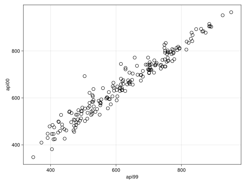

source

Survey.boxplot — Function

boxplot(design, x, y; kwargs...)

Box plot of survey design variable y grouped by column x.

Weights can be specified by a Symbol using the keyword argument weights.

The keyword arguments are all the arguments that can be passed to mapping in AlgebraOfGraphics.

julia> using AlgebraOfGraphics

julia> apisrs = load_data("apisrs");

julia> srs = SurveyDesign(apisrs; weights=:pw);

julia> bp = boxplot(srs, :stype, :enroll; weights = :pw);

julia> save("boxplot.png", bp)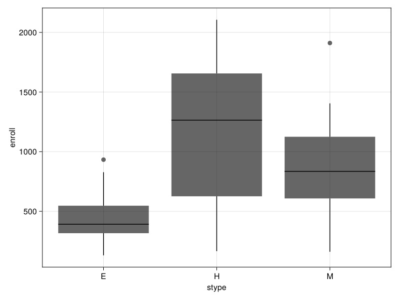

source

Survey.hist — Function

hist(design, var, bins = freedman_diaconis; normalization = :density, kwargs...)

Histogram plot of a survey design variable given by var.

bins can be an Integer specifying the number of equal-width bins, an AbstractVector specifying the bins intervals, or a Function specifying the function used for calculating the number of bins. The possible functions are sturges and freedman_diaconis.

The normalization can be set to :none, :density, :probability or :pdf. See AlgebraOfGraphics.histogram for more information.

For the complete argument list see Makie.hist.

Note

The weights argument should be a Symbol specifying a design variable.

julia> using AlgebraOfGraphics

julia> apisrs = load_data("apisrs");

julia> srs = SurveyDesign(apisrs; weights=:pw);

julia> h = hist(srs, :enroll);

julia> save("hist.png", h)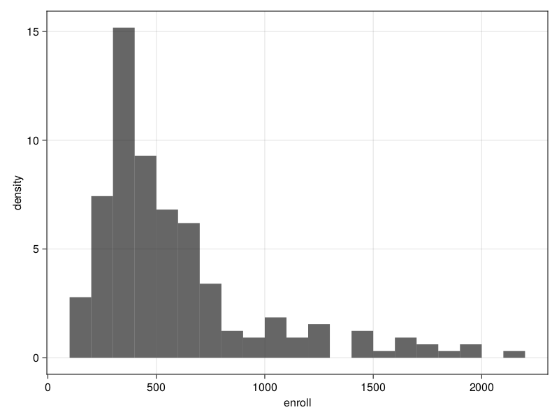

source

Survey.sturges — Function

sturges(design::SurveyDesign, var::Symbol)

Calculate the number of bins to use in a histogram using the Sturges rule.

Examples

julia> apisrs = load_data("apisrs");

julia> srs = SurveyDesign(apisrs; weights=:pw);

julia> sturges(srs, :enroll)
9

source

Survey.freedman_diaconis — Function

freedman_diaconis(design::SurveyDesign, var::Symbol)

Calculate the number of bins to use in a histogram using the Freedman-Diaconis rule.

Examples

julia> apisrs = load_data("apisrs");

julia> srs = SurveyDesign(apisrs; weights=:pw);

julia> freedman_diaconis(srs, :enroll)
18

source