Installation
The Survey.jl package is registered. Regular Pkg commands can be used for installing the package:
julia> using Pkgjulia> Pkg.add("Survey")Updating registry at `~/.julia/registries/General.toml` Resolving package versions... Installed Survey ─ v0.2.0 Updating `~/work/Survey.jl/Survey.jl/docs/Project.toml` [c1a98b4d] ~ Survey v0.3.0 `~/work/Survey.jl/Survey.jl` ⇒ v0.2.0 Updating `~/work/Survey.jl/Survey.jl/docs/Manifest.toml` [c1a98b4d] ~ Survey v0.3.0 `~/work/Survey.jl/Survey.jl` ⇒ v0.2.0 Precompiling project... ✓ UnPack ✓ RangeArrays ✓ PositiveFactorizations ✓ PkgVersion ✓ Grisu ✓ MappedArrays ✓ Inflate ✓ ProgressMeter ✓ CommonSubexpressions ✓ DiffResults ✓ SimpleTraits ✓ StackViews ✓ Imath_jll ✓ PaddedViews ✓ LLVMOpenMP_jll ✓ IntelOpenMP_jll ✓ JpegTurbo_jll ✓ ArrayInterface ✓ Parameters ✓ DiffRules ✓ QOI ✓ MosaicViews ✓ OpenEXR_jll ✓ AxisArrays ✓ MKL_jll ✓ libsixel_jll ✓ ArrayInterface → ArrayInterfaceGPUArraysCoreExt ✓ ArrayInterface → ArrayInterfaceStaticArraysCoreExt ✓ OpenEXR ✓ FiniteDiff ✓ FiniteDiff → FiniteDiffStaticArraysExt ✓ ForwardDiff ✓ ForwardDiff → ForwardDiffStaticArraysExt ✓ NLSolversBase ✓ LineSearches ✓ Optim ✓ ImageCore ✓ JpegTurbo ✓ Sixel ✓ ImageBase ✓ PNGFiles ✓ ImageAxes ✓ ImageMetadata ✓ Netpbm ✓ TiffImages ✓ Survey 46 dependencies successfully precompiled in 61 seconds. 238 already precompiled. 1 dependency precompiled but a different version is currently loaded. Restart julia to access the new version
] add SurveyTutorial
This tutorial assumes basic knowledge of statistics and survey analysis.
To begin this tutorial, load the package in your workspace:
julia> using Survey
Now load a survey dataset that you want to study. In this tutorial we will be using the Academic Performance Index (API) datasets for Californian schools. The datasets contain information for all schools with at least 100 students and for various probability samples of the data.
julia> apisrs = load_data("apisrs")200×40 DataFrame
 Row │ Column1  cds             stype    name             sname                ⋯
     │ Int64    Int64           String1  String15         String               ⋯
─────┼──────────────────────────────────────────────────────────────────────────
   1 │    1039  15739081534155  H        McFarland High   McFarland High       ⋯
   2 │    1124  19642126066716  E        Stowers (Cecil   Stowers (Cecil B.) E
   3 │    2868  30664493030640  H        Brea-Olinda Hig  Brea-Olinda High
   4 │    1273  19644516012744  E        Alameda Element  Alameda Elementary
   5 │    4926  40688096043293  E        Sunnyside Eleme  Sunnyside Elementary ⋯
   6 │    2463  19734456014278  E        Los Molinos Ele  Los Molinos Elementa
   7 │    2031  19647336058200  M        Northridge Midd  Northridge Middle
   8 │    1736  19647336017271  E        Glassell Park E  Glassell Park Elemen
  ⋮  │    ⋮           ⋮            ⋮            ⋮                       ⋮      ⋱
 194 │    4880  39686766042782  E        Tyler Skills El  Tyler Skills Element ⋯
 195 │     993  15636851531987  H        Desert Junior/S  Desert Junior/Senior
 196 │     969  15635291534775  H        North High       North High
 197 │    1752  19647336017446  E        Hammel Street E  Hammel Street Elemen
 198 │    4480  37683386039143  E        Audubon Element  Audubon Elementary   ⋯
 199 │    4062  36678196036222  E        Edison Elementa  Edison Elementary
 200 │    2683  24657716025621  E        Franklin Elemen  Franklin Elementary
                                                 36 columns and 185 rows omitted
apisrs is a simple random sample of the Academic Performance Index of Californian schools. The load_data function loads it as a DataFrame. You can look at the column names of apisrs to get an idea of what the dataset contains.
julia> names(apisrs)40-element Vector{String}:
 "Column1"
 "cds"
 "stype"
 "name"
 "sname"
 "snum"
 "dname"
 "dnum"
 "cname"
 "cnum"
 ⋮
 "col.grad"
 "grad.sch"
 "avg.ed"
 "full"
 "emer"
 "enroll"
 "api.stu"
 "pw"
 "fpc"
Next, build a survey design from your DataFrame:
julia> srs = SurveyDesign(apisrs; weights=:pw)SurveyDesign:
data: 200×45 DataFrame
strata: none
cluster: none
popsize: [6194.0, 6194.0, 6194.0  …  6194.0]
sampsize: [200, 200, 200  …  200]
weights: [30.97, 30.97, 30.97  …  30.97]
allprobs: [0.0323, 0.0323, 0.0323  …  0.0323]
This is a simple random sample design with weights given by the column :pw of apisrs. You can also create more complex designs such as stratified or cluster sample designs. You can find more information on the complete capabilities of the package in the Manual. The purpose of this tutorial is to show the basic usage of the package. For that, we will stick with a simple random sample.
Now you can analyse your design according to your needs using the functionality provided by the package. For example, you can compute the estimated mean or population total for a given variable. Let's say you want to find the mean Academic Performance Index from the year 1999. If you are only interested in the estimated mean, then you can directly pass your design to the mean function:
julia> mean(:api99, srs)1×1 DataFrame
 Row │ mean
     │ Float64
─────┼─────────
   1 │ 624.685
If you also want to know the standard error of the mean, you need to convert the SurveyDesign to a ReplicateDesign using bootstrapping:
julia> bsrs = bootweights(srs; replicates = 1000)ReplicateDesign{BootstrapReplicates}: data: 200×1045 DataFrame strata: none cluster: none popsize: [6194.0, 6194.0, 6194.0 … 6194.0] sampsize: [200, 200, 200 … 200] weights: [30.97, 30.97, 30.97 … 30.97] allprobs: [0.0323, 0.0323, 0.0323 … 0.0323] type: bootstrap replicates: 1000julia> mean(:api99, bsrs)1×2 DataFrame Row │ mean SE │ Float64 Float64 ─────┼────────────────── 1 │ 624.685 9.84669
You can find the mean of both the 1999 API and 2000 API for a clear comparison between students' performance from one year to another:
julia> mean([:api99, :api00], bsrs)2×3 DataFrame
 Row │ names   mean     SE
     │ String  Float64  Float64
─────┼──────────────────────────
   1 │ api99   624.685  9.84669
   2 │ api00   656.585  9.5409
The ratio is also appropriate for studying the relationship between the two APIs:
julia> ratio(:api00, :api99, bsrs)ERROR: MethodError: no method matching ratio(::Symbol, ::Symbol, ::ReplicateDesign{BootstrapReplicates})

Closest candidates are:
  ratio(::Vector{Symbol}, ::Any, ::AbstractSurveyDesign)
   @ Survey ~/work/Survey.jl/Survey.jl/src/ratio.jl:109
If you're interested in a certain statistic estimated by a specific domain, you can add the domain as the second parameter to your function. Let's say you want to find the estimated total number of students enrolled in schools from each county:
julia> total(:enroll, :cname, bsrs)38×3 DataFrame
 Row │ total           SE             cname
     │ Float64         Float64        String
─────┼────────────────────────────────────────────────
   1 │      1.95823e5  74731.2        Kern
   2 │ 867129.0            1.36622e5  Los Angeles
   3 │      1.68786e5  63858.0        Orange
   4 │   6720.49        6790.49       San Luis Obispo
   5 │  30319.6        18197.6        San Francisco
   6 │   6503.7         6481.36       Modoc
   7 │ 134224.0        46808.0        Alameda
   8 │  64479.5        39542.0        Solano
  ⋮  │       ⋮               ⋮               ⋮
  32 │  32642.4        23541.9        Kings
  33 │  36203.9        32062.1        Shasta
  34 │  12171.2        12502.9        Yolo
  35 │  12976.4        13241.6        Calaveras
  36 │  39239.0        30181.9        Napa
  37 │   6410.79        6986.29       Lake
  38 │  15392.1        15202.2        Merced
                                       23 rows omitted
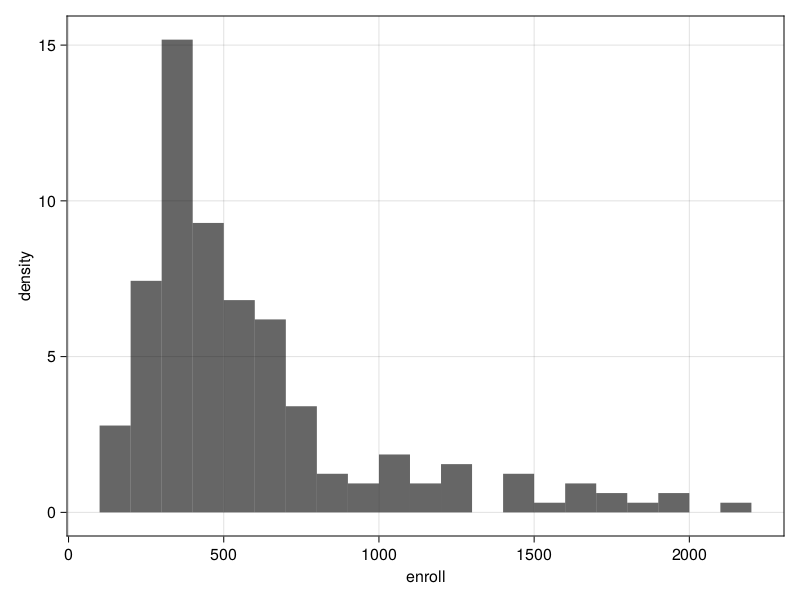
Another way to visualize data is through graphs. You can make a histogram to better see the distribution of enrolled students:
julia> hist(srs, :enroll)The REPL doesn't show the plot. To see it, you need to save it locally.
julia> import AlgebraOfGraphics.save

julia> save("hist.png", h)